Centralized vs Distributed Splitting in PON: Which Architecture Fits Your FTTH Network?
By Jergeo Engineering Team | Published September 2026 · 14 min read
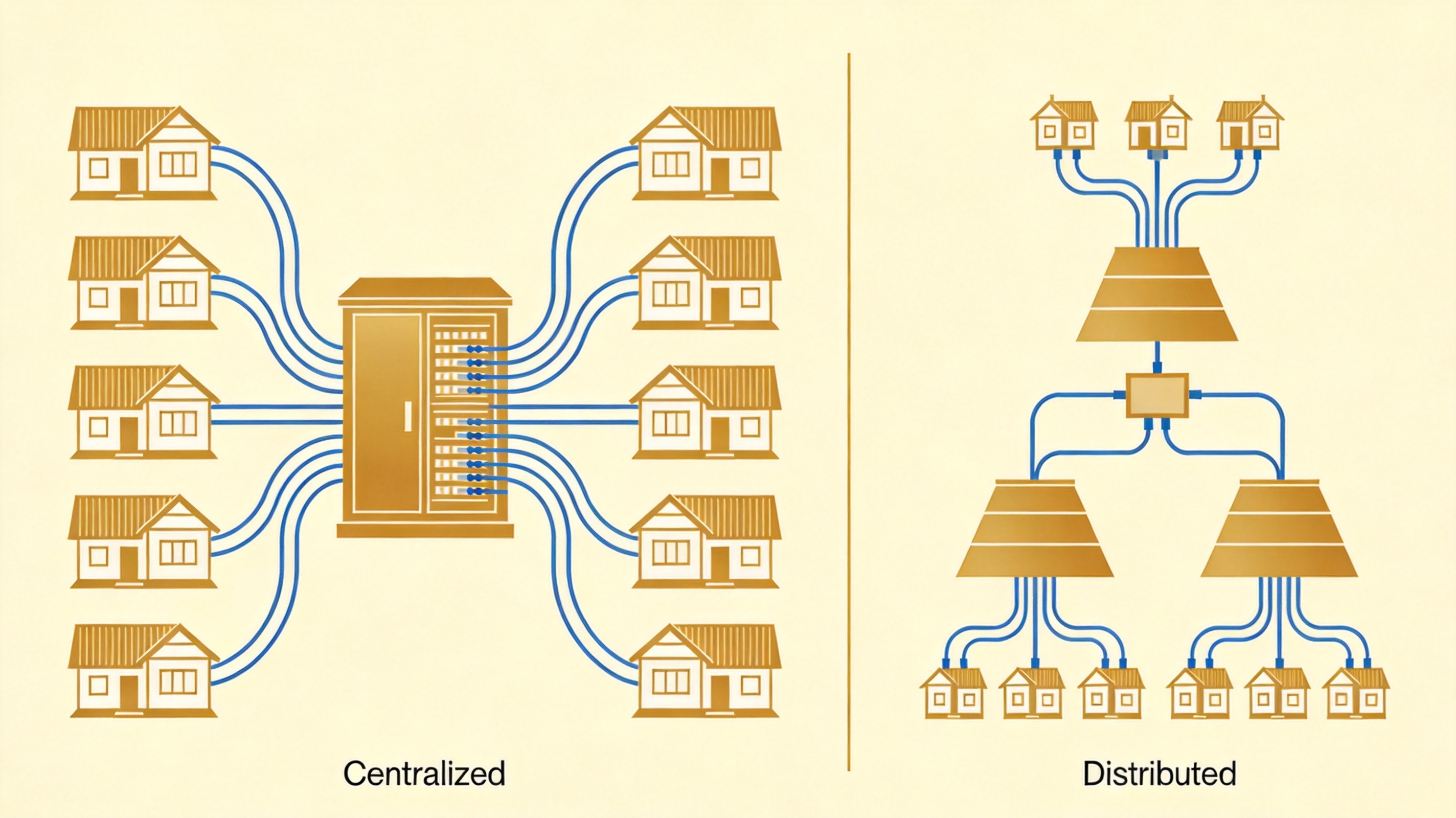
When you design a PON-based FTTH network, the single most consequential passive infrastructure decision isn't which fiber cable to buy or which connector polish to specify. It's where you put the splitters. Centralized or distributed? This choice determines how much fiber you bury, how many cabinets you install, how efficiently your OLT ports get used, and how painful future upgrades will be. Get it wrong, and you're either over-building with fiber you don't need — or struggling with OLT port exhaustion and truck rolls that never stop.
Summary
Centralized splitting puts all splitters in one location (a cabinet or FDH), maximizing OLT port utilization and simplifying maintenance — at the cost of significantly more distribution fiber. Distributed (cascaded) splitting stages the split across two or more locations, reducing fiber requirements and shortening drop distances — but adding maintenance complexity and cumulative insertion loss. The right choice depends on subscriber density, take-rate expectations, geography, and your CAPEX vs OPEX priorities. In practice, many operators use a hybrid of both.
TL;DR
Centralized splitting puts all splitters in one location (a cabinet or FDH), maximizing OLT port utilization and simplifying maintenance — at the cost of significantly more distribution fiber. Distributed (cascaded) splitting stages the split across two or more locations, reducing fiber requirements and shortening drop distances — but adding maintenance complexity and cumulative insertion loss. The right choice depends on subscriber density, take-rate expectations, geography, and your CAPEX vs OPEX priorities. In practice, many operators use a hybrid of both.
How PON Splitting Works: The Basics
In a passive optical network, a single OLT port serves multiple subscribers through passive optical splitters. The splitter divides one optical signal into N equal outputs — and each output can either go directly to a subscriber, or feed another splitter downstream. The total split ratio (e.g., 1:32) determines how many ONUs share one OLT port and how much bandwidth each gets.
The question is not how much total splitting you need — that's a business decision based on subscriber count and service tier. The question is where physically that splitting happens in the network topology. And that's where centralized and distributed architectures diverge.
Centralized Splitting: One Location, All Splitters
In a centralized splitting architecture, all passive splitters are co-located at a single point — typically a fiber distribution cabinet, a fiber distribution hub (FDH), or the central office itself. The OLT port connects to one high-ratio splitter (1:32 or 1:64), and individual fiber strands run from that splitter to each subscriber premises.
How it works in practice
The OLT port in the central office connects to a fiber that leaves the CO and reaches the input port of a splitter, typically housed in a street-side cabinet. For a 1:64 configuration, this might be a single 1:64 splitter, or a combination like 1:2 at the CO feeding 1:32 in the cabinet. The splitter's output ports fan out through the distribution network, reaching homes through closures and terminal boxes.
The key characteristic: one physical location handles all the splitting for an entire PON tree. Every subscriber's fiber trace passes through that single cabinet.
Why operators choose centralized splitting
- OLT port utilization. A centralized 1:32 splitter concentrates 200 potential subscribers onto 32 active OLT ports. In early deployment phases with low take rates (20–40%), you only activate the ports you need. As subscriptions grow, you fill ports without touching the field plant. See CommScope's FTTH planning white paper for detailed analysis.
- Single-point maintenance. All splitters in one cabinet means one location for testing, reconfiguration, and troubleshooting. An OTDR trace from the FDH can characterize every downstream branch. Fewer truck rolls, simpler record keeping.
- Technology flexibility. Connectorized single-stage splitters can be swapped out when upgrading from GPON to XGS-PON or WDM-PON — without disturbing the distribution fiber plant. The ODN stays; only the active equipment and splitter cassettes change.
Where it hurts
- More distribution fiber. Every subscriber gets a dedicated fiber from the centralized splitter location. For 200 homes served by a 1:32 splitter, you still need 200 individual fiber runs from the cabinet to the premises — even though only 32 are active initially. CommScope estimates this can increase distribution cable CAPEX by over 38% compared to cascaded topologies.
- Larger outdoor cabinets. A 1:64 splitter with 64 terminated outputs requires a substantial cabinet — more expensive, more street real estate, more likely to trigger local planning permits.
- Longer drop distances. When all splitting is centralized, the average distance from the splitter to each subscriber increases, especially in sprawling layouts. Longer drops mean more fiber per subscriber and higher attenuation.
Distributed (Cascaded) Splitting: Two or More Stages
In a distributed splitting architecture, the total split ratio is achieved across multiple stages at different physical locations. The most common configuration is two-stage: a first-stage splitter (1:4 or 1:8) near the central office, feeding second-stage splitters (1:8 or 1:16) in terminal boxes close to subscriber clusters.
How it works in practice
The OLT port connects directly to an outside plant fiber — no splitter at the central office. A first-level splitter (say, 1:4) sits in a closure not far from the CO. Each of the four outputs runs to a different neighborhood area, where a second-level splitter (1:8) in a terminal box serves 8 homes. The combined ratio: 1:4 × 1:8 = 1:32. Same total split, different physical layout.
Why operators choose distributed splitting
- Significantly less distribution fiber. Instead of running individual fibers from a central point to every subscriber, the second-stage splitters sit close to subscriber clusters. Drop distances shrink to tens of meters. Research indicates distributed architectures can reduce FDH cabinet capacity by up to 75% and cut distribution fiber counts proportionally.
- Lower initial CAPEX on fiber. Less fiber in the distribution plant — the most expensive OSP component — means lower upfront investment. This matters most when civil works (trenching, ducting) are needed, because fewer fibers = smaller ducts = lower digging costs.
- Shorter subscriber drops. When a technician connects a new customer, the drop runs from a terminal box tens of meters away — not hundreds of meters from a distant cabinet. All service turn-up work happens at the premises, without a second trip to a remote splitter cabinet.
Where it hurts
- Lower OLT port utilization at low take rates. In a distributed architecture, the second-stage splitters are deployed regardless of local take rate. If a 1:8 splitter serves 8 homes but only 2 are active, the OLT port sees 2/32 utilization — the other 30 potential ports on the PON are stranded. This is the inverse of centralized splitting's efficiency advantage.
- More field locations to maintain. Multiple splitter locations across the network means more points of failure, more records to maintain, and more truck rolls when something goes wrong. A fault in a second-stage splitter requires finding the right field enclosure — which may be a pole-mounted closure or underground pedestal.
- Higher cumulative insertion loss. This is the one most guides understate — and it's the focus of the next section.
The Real Trade-Off: Cumulative Insertion Loss
This is where physics meets economics. Two-stage splitting doesn't just add two splitters — it adds the insertion loss of both splitters plus the extra connectors and splices between them.
| Component | Centralized 1:32 | Distributed 1:4 + 1:8 |
|---|---|---|
| Splitter insertion loss | ≈ 16.9 dB | 7.1 + 10.5 = 17.6 dB |
| Extra connector pairs (2 stages) | Included above | + 0.6 dB (2 pairs × 0.3 dB) |
| Extra splices (2 stages) | Included above | + 0.2 dB (2 × 0.1 dB) |
| Total passive loss | ≈ 16.9 dB | ≈ 18.4 dB |
| Penalty | Distributed consumes ~1.5 dB more margin → ~4-5 km less reach at 0.35 dB/km | |
On a GPON Class B+ system with a 28 dB power budget, that 1.5 dB penalty is the difference between comfortably reaching subscribers 20 km away and falling short. On longer rural feeder runs, it can push distant subscribers below the ONT receiver threshold — forcing you to either reduce the split ratio (fewer subscribers per OLT port) or add an active repeater (defeating the purpose of a passive network).
For a detailed walkthrough of power budget calculations, see our fiber optic power budget guide.
When to Choose Which: A Decision Framework
Choose centralized splitting when:
- Subscriber density is high (urban areas, MDU buildings, business districts). The fiber cost penalty is smaller when drops are short anyway, and OLT efficiency pays off quickly as take rates climb.
- Take rates are expected to be high or fast-growing. If you expect 50%+ activation within the first year, centralized splitting's port utilization advantage kicks in fast.
- Maintenance simplicity is a priority. Single-location access means fewer truck rolls and faster fault resolution — important in areas where field access is difficult or expensive.
- Technology upgrades are on the roadmap. Connectorized centralized splitters swap out cleanly when migrating from GPON to XGS-PON or NG-PON2.
Choose distributed splitting when:
- Subscriber density is low (rural and suburban areas, dispersed communities). The fiber savings are massive — you avoid running hundreds of individual fibers from a distant cabinet to widely scattered homes.
- Initial take rates are low. If you expect 20–30% activation in year one, distributed splitting defers second-stage infrastructure investment until demand materializes.
- Civil works costs dominate. When trenching costs $50–150 per meter, reducing fiber count directly reduces duct size and excavation expense. The 38%+ fiber savings from centralized splitting becomes an expensive luxury.
- Drop distances from a central point would be excessive. In sprawling layouts, centralized splitting can force subscriber drops of 500+ meters — more fiber per subscriber, more attenuation, more cost.
Consider a hybrid approach when:
Most real-world FTTH networks aren't purely one or the other. A common hybrid pattern: centralized primary splits at the FDH for dispersed residential zones (simplicity and OLT efficiency), with distributed secondary splits for MDU clusters or dense suburban pockets (fiber savings and shorter drops). This is particularly common in BEAD-funded rural builds where subscriber density varies across the service area.
How Splitting Architecture Drives Equipment Selection
Your splitting architecture decision directly determines which enclosure types and splitter form factors you'll purchase in volume. Planning one without the other is how projects end up with the right splitter chip in the wrong housing.
| Architecture | Splitter Form Factor | Enclosure Type | Why |
|---|---|---|---|
| Centralized | LGX cassette or 1U rack-mount | Large street cabinet or FDH | High port density at one location; front-panel access for testing and reconfiguration |
| Distributed (Stage 1) | LGX cassette or tray-type | Medium cabinet or equipment room | First-stage split near CO; moderate port count |
| Distributed (Stage 2) | ABS box or blockless | Small closure or terminal box | Outdoor environment, close to subscribers; weatherproof required |
Jergeo supplies equipment across both architectures:
- For centralized architectures: JFDC-288A outdoor fiber distribution cabinet (288 ports, IP65, SMC) houses high-ratio splitters with organized fiber management. Combined with 1x32 tray-type PLC splitter cassettes (SC/LC, PC/UPC/APC polish).
- For distributed architectures: JFDB-64A fiber distribution box (IP65, outdoor-rated) serves as second-stage enclosure near subscriber clusters, with 1x8 card-type PLC splitter cassettes for the final distribution stage.
Five Mistakes We've Seen in the Field
- Choosing architecture before understanding take rate. The most common error. If you assume 60% take rate and design centralized, but actual activation is 20%, you're paying for stranded OLT ports. Model conservative scenarios first.
- Ignoring the 1.5 dB penalty in distributed designs. Teams calculate split ratio loss correctly but forget the extra connectors and splices between stages. On a 20 km rural feeder, that missing 1.5 dB can strand the farthest subscribers.
- Specifying centralized cabinets too small. A 1:64 splitter with 64 pigtails and splice trays needs more physical space than planners expect. Always spec cabinets with 20–30% spare capacity for future expansion.
- Using the wrong splitter packaging for the environment. Putting indoor-rated ABS box splitters in outdoor closures, or using bare blockless splitters in cabinets that need front-panel accessibility. The splitting architecture determines which packaging you need — plan them together.
- No documentation for distributed splitter locations. With centralized splitting, everything is in one cabinet. With distributed, you have multiple field locations that must be mapped, labeled, and tracked. Inadequate records turn every fault into a scavenger hunt.
The Bottom Line
There is no universally superior architecture. Centralized splitting optimizes OPEX (easy management, simple troubleshooting, efficient OLT utilization) at the cost of higher CAPEX (more fiber, larger cabinets). Distributed splitting inverts that trade-off — lower fiber CAPEX, but more field locations and cumulative loss. The skill is matching architecture to your specific deployment scenario: subscriber density, geography, budget, and growth expectations.
The best architecture is the one that reduces capital expense, optimizes long-term operational expense, and creates a future-proof network that can adapt to new technologies without dramatic rebuilds. For most operators, that means evaluating both options against real subscriber data — not assumptions.
A note on accuracy. The loss values, cost comparisons, and architecture recommendations in this guide are compiled from CommScope's FTTH planning white papers, Draftech's GPON network design guide, and multiple engineering field references. Actual performance depends on specific components, installation quality, and local conditions. For precise optical loss calculations, refer to the datasheets of the specific splitters and cables you deploy.
Related Products
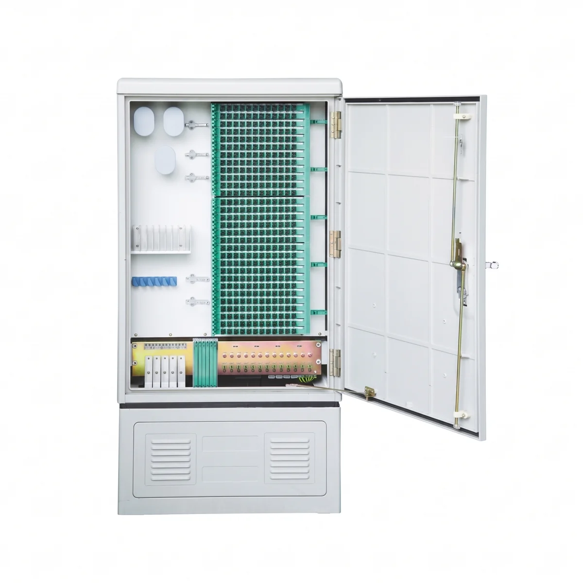
JFDC-288A Outdoor Cabinet
288 ports, IP65, SMC enclosure — ideal central point for concentrated splitter deployment
View Product →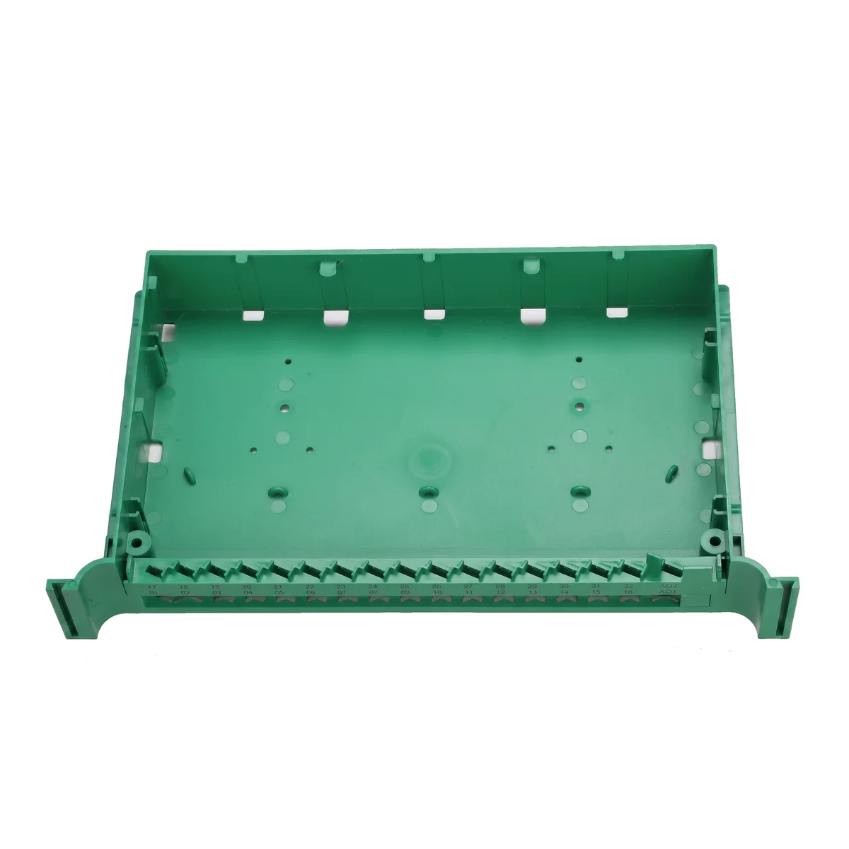
JPLCT-32A 1×32 Tray Cassette
Tray-type 1:32 PLC splitter, SC/LC connectors, −40 to +85°C for cabinet-mounted splitting
View Product →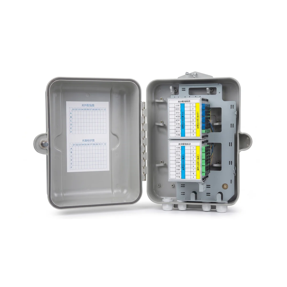
JFDB-64A Outdoor FDB
IP65-rated distribution box for second-stage splitting near subscriber clusters
View Product →Related Articles

Fiber Optic Splitter Guide
PLC vs FBT, form factors, connector options — how splitter packaging choices follow from your architecture decision.
Read Article →
FTTH Network Architecture Guide
The full ODN hierarchy — where splitters, cabinets, and distribution boxes fit in the end-to-end topology.
Read Article →
Fiber Distribution Cabinet Buying Guide
Capacity planning, IP rating, splitter integration — selecting the right cabinet for your splitting architecture.
Read Article →